t-tests
Lecture 06
Dr Jennifer Mankin
5 March 2021

Looking Ahead (and Behind)
Week 4: Correlation
Last week: Chi-Square ( )
Looking Ahead (and Behind)
Week 4: Correlation
Last week: Chi-Square ( )
This week: t-test
Looking Ahead (and Behind)
Week 4: Correlation
Last week: Chi-Square ( )
This week: t-test
Next week: The Linear Model
Week 8: The Linear Model
Lab Report: Red Study
Today we will talk about one of the analyses for the lab report
: Green study (Griskevicious et al., 2010), last week
t-test: Red study (Elliot et al., 2020), today!
We will talk about the lab report in the lectures and work on it in the practicals
- Make sure you come to your registered sessions
Objectives
After this lecture you will understand:
The concepts behind comparing two means
- Independent and paired samples t-tests
Where the t-statistic comes from
How to read histograms and means plots
How to interpret and report significance tests of t
Comparing Two Means
Extremely common and fundamental testing paradigm
Comparing means in two groups
Independent: different entities/participants in each groups
Paired: same entities/participants in both groups
Very similar logic and interpretation, slightly different maths!
Taste the Rainbow: Synaesthesia Again
People with synaesthesia have unusual sensory experiences
- Experience colours for words, shapes for music, personalities for numbers, etc.
Grapheme-Colour Synaesthesia
Association between letters/words and particular colours
Tends to be consistent throughout life, beginning in childhood
So, synaesthetes might tend to notice language/spelling more often
Research question: Do synaesthetes have a particular cognitive style, compared to non-synaesthetes?
Conceptual hypothesis: grapheme-colour synaesthetes have a more language-oriented cognitive style than non-synaesthetes
Data and Design: SCSQ
Mealor et al (2016): Sussex Cognitive Styles Questionnaire
Includes measures of imagery, language ability, and more
Validated on people with and without synaesthesia
Data and Design: SCSQ
Mealor et al (2016): Sussex Cognitive Styles Questionnaire
Includes measures of imagery, language ability, and more
Validated on people with and without synaesthesia
Operational hypothesis: Synaesthetes will, on average, have a different score on the Language subscale of the SCSQ than non-synaesthetes
- Example items: "I tend to notice if a word has the same letter repeated in its spelling"; "I enjoy learning new languages"
Null hypothesis: Synaesthetes and non-synaesthetes will, on average, have the same score on the Language subscale
Having a Look
- All scores on the Language subscale together
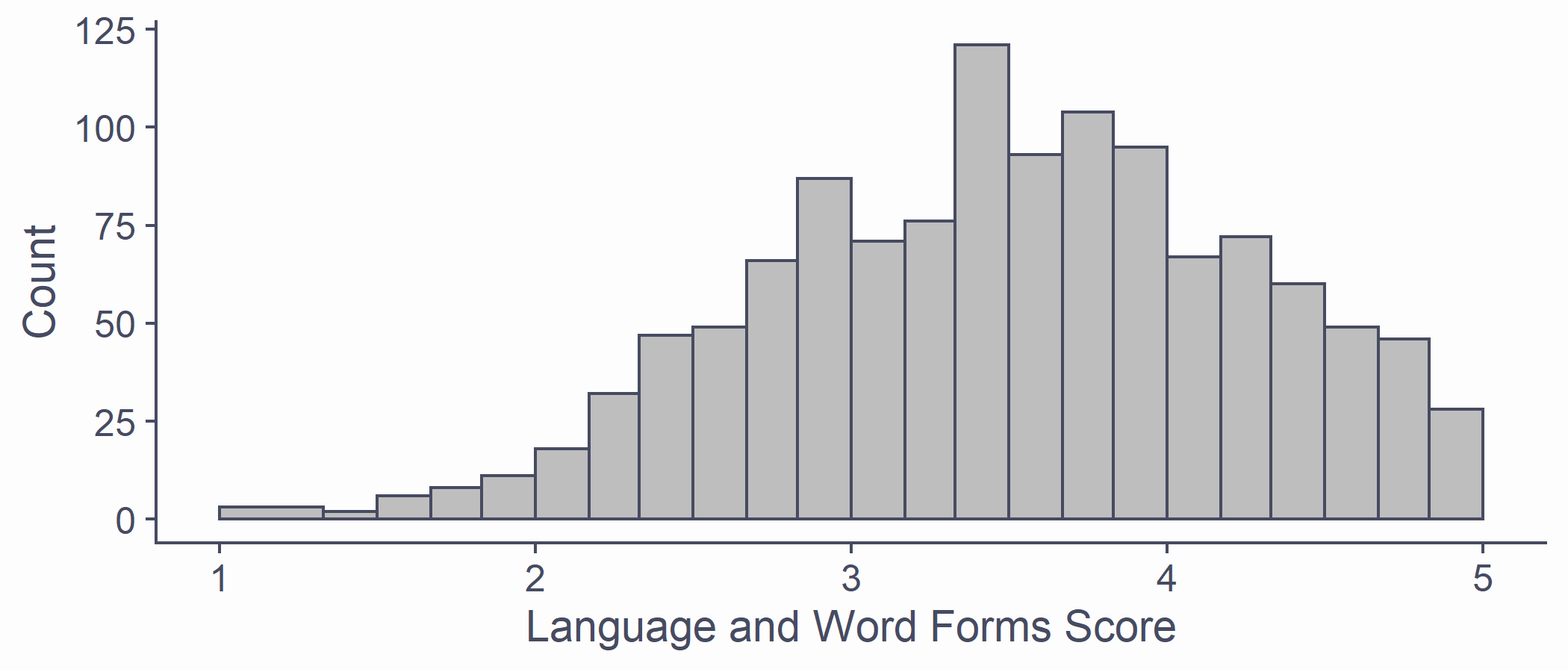
syn_data %>% ggplot(aes(x = Language)) + geom_histogram(breaks = syn_data %>% pull(Language) %>% unique(), fill = "grey") + scale_x_continuous(name = "Language and Word Forms Score", limits = c(1, 5)) + scale_y_continuous(name = "Count")Having a Look
- Split up by grapheme-colour synaesthesia
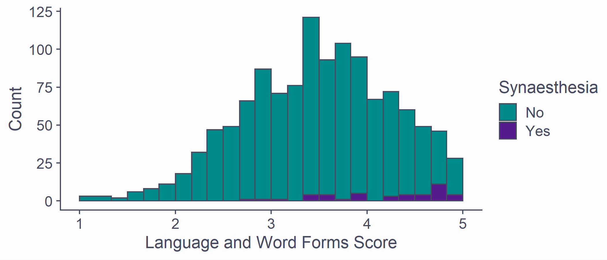
syn_data %>% ggplot(aes(x = Language, fill = GraphCol)) + geom_histogram(breaks = syn_data %>% pull(Language) %>% unique()) + scale_x_continuous(name = "Language and Word Forms Score", limits = c(1, 5)) + scale_y_continuous(name = "Count") + scale_fill_discrete(name = "Synaesthesia", type = c("darkcyan", "purple4"))Having a Look
- Dotted lines for mean scores in each group
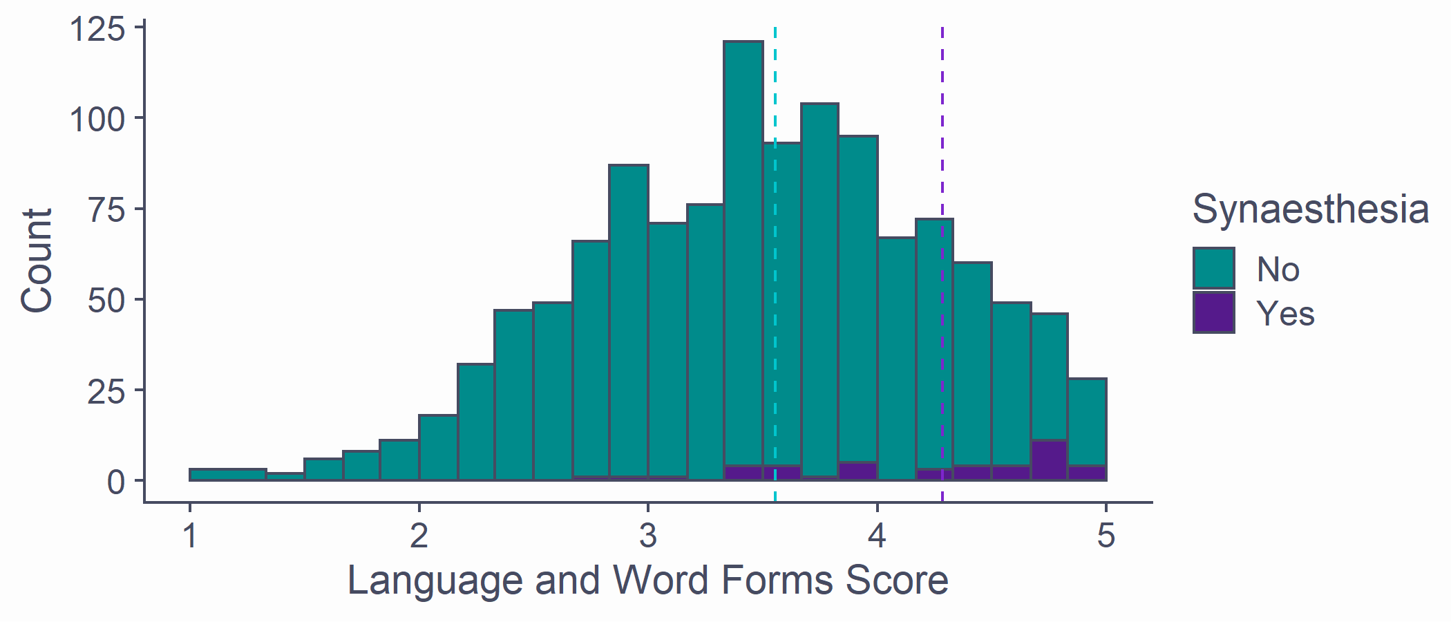
syn_data %>% ggplot(aes(x = Language, fill = GraphCol)) + geom_histogram(breaks = syn_data %>% pull(Language) %>% unique()) + scale_x_continuous(name = "Language and Word Forms Score", limits = c(1, 5)) + scale_y_continuous(name = "Count") + scale_fill_discrete(name = "Synaesthesia", type = c("darkcyan", "purple4")) + geom_vline(aes(xintercept = mean(Language)), data = syn_data %>% filter(GraphCol == "Yes"), colour = "purple3", linetype = "dashed") + geom_vline(aes(xintercept = mean(Language)), data = syn_data %>% filter(GraphCol == "No"), colour = "turquoise3", linetype = "dashed")Sorted!
The mean Language score for synaesthetes is higher than for non-synaesthetes
Are we done?
Sorted!
The mean Language score for synaesthetes is higher than for non-synaesthetes
Are we done?
Of course not 😉
How different are these mean scores, accounting for the variation in scores?
How strong is the signal (the difference in means)...
Compared to the noise (the variation in scores around the mean)?
Having a Closer Look
Plot of the means in each group
- Error bars represent 2 the standard error
How can we interpret this plot?
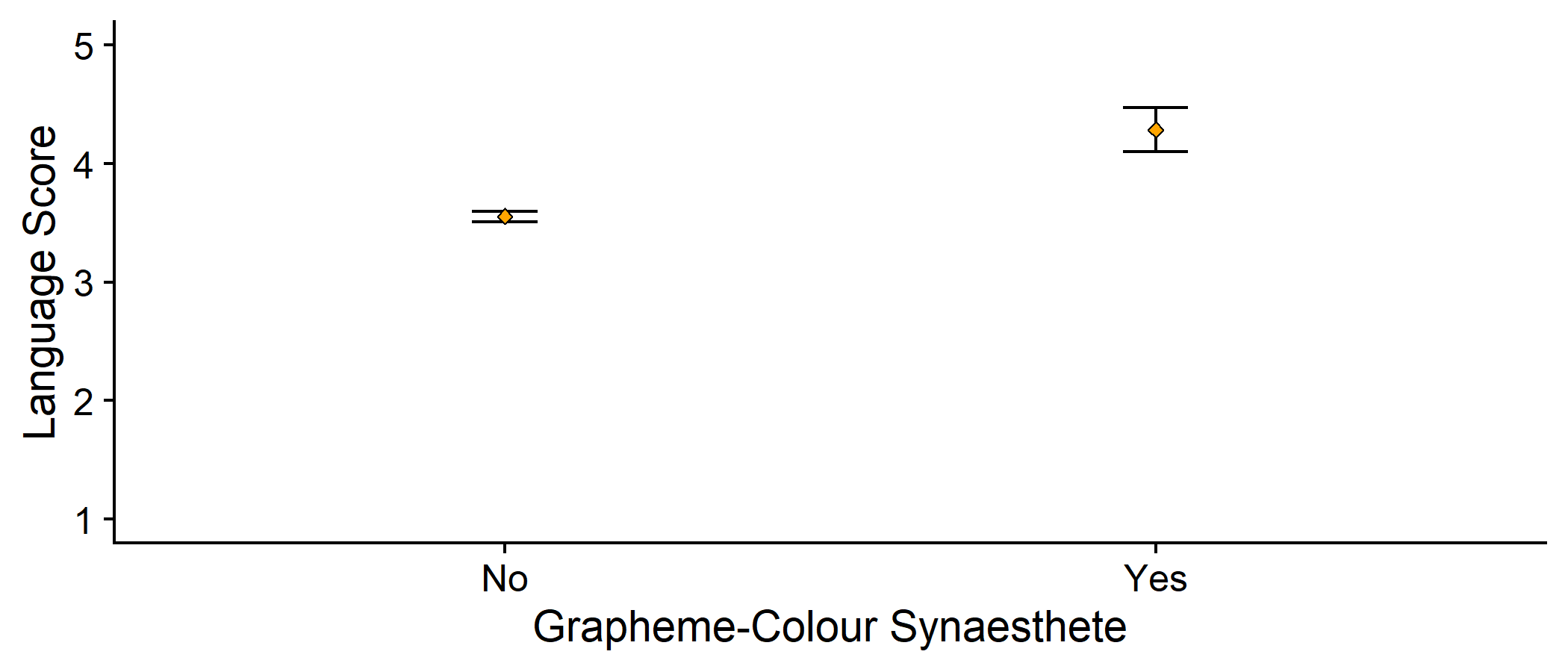
syn_data %>% dplyr::group_by(GraphCol) %>% dplyr::summarise( n = dplyr::n(), mean_lang = mean(Language), se_lang = sd(Language)/sqrt(n) ) %>% ggplot2::ggplot(aes(x = GraphCol, y = mean_lang)) + geom_errorbar(aes(ymin = mean_lang - 2*se_lang, ymax = mean_lang + 2*se_lang), width = .1) + geom_point(colour = "black", fill = "orange", pch = 23) + scale_y_continuous(name = "Language Score", limits = c(1, 5)) + labs(x = "Grapheme-Colour Synaesthete") + cowplot::theme_cowplot()Why You Gotta Be So Mean
Let's get some numbers to work with 😁
Mean in synaesthete group: 4.29
Mean in nonsynaesthete group: 3.55
Why You Gotta Be So Mean
Let's get some numbers to work with 😁
Mean in synaesthete group: 4.29
Mean in nonsynaesthete group: 3.55
Difference in the means = 4.29 - 3.55 = 0.74
Why You Gotta Be So Mean
Let's get some numbers to work with 😁
Mean in synaesthete group: 4.29
Mean in nonsynaesthete group: 3.55
Difference in the means = 4.29 - 3.55 = 0.74
Is this a big difference, compared to how different we might expect for any two sample means from the same population?
Steps of the Analysis
- Calculate the (standardised) difference between mean scores
Steps of the Analysis
Calculate the (standardised) difference between mean scores
Compare that test statistic to its distribution under the null hypothesis
Steps of the Analysis
Calculate the (standardised) difference between mean scores
Compare that test statistic to its distribution under the null hypothesis
Obtain the probability p of encountering a test statistic of the size we have, or larger, if the null hypothesis is true
Steps of the Analysis
Calculate the (standardised) difference between mean scores
Compare that test statistic to its distribution under the null hypothesis
Obtain the probability p of encountering a test statistic of the size we have, or larger, if the null hypothesis is true
## ## Two Sample t-test## ## data: Language by GraphCol## t = -6.3394, df = 1209, p-value = 0.000000000325## alternative hypothesis: true difference in means is not equal to 0## 95 percent confidence interval:## -0.9576637 -0.5049972## sample estimates:## mean in group No mean in group Yes ## 3.554949 4.286279- Where does this number t come from? And what does it mean?
Let's Think About This
Imagine we took two samples of scores from a single population and calculated their means, and then found the difference between those means
Create a sampling distribution of mean differences
Centre of the distribution = 0 (no difference between the means)
Very small differences in means will be quite common
Very large differences in means will be quite unlikely
Distribution under the null hypothesis that which group you're in (e.g. synaesthete vs non-synaesthete) makes no difference to your score
- Samples come from the same population of scores
Sound Familiar?
If this rings a bell, it should!
- This is the same scenario from Lecture 3 for the Ape Index (AI)
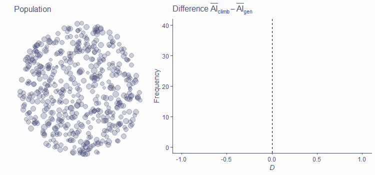
Sound Familiar?
Our estimate of mean Language score difference (0.74) also has some distribution
- Using that distribution, obtain the probability p of finding a difference as large as the one we found, or larger, if the null hypothesis is true (as usual)
Sound Familiar?
Our estimate of mean Language score difference (0.74) also has some distribution
- Using that distribution, obtain the probability p of finding a difference as large as the one we found, or larger, if the null hypothesis is true (as usual)
Standardise our mean difference to compare it to a known distribution
We can do this by dividing the mean difference by the standard error
In other words: scale it to the distribution
Conceptually similar to z-scores
Same But Different
For the AI in Lecture 3, the standard deviation of the population was 1
Assumed for simplicity
Remember,
Same But Different
For the AI in Lecture 3, the standard deviation of the population was 1
Assumed for simplicity
Remember,
For our synaesthesia example, the standard error is a variable
We estimate based on the standard deviation s
Every sample, even samples of the same size, will have a different s!
What's the Point?
The test statistic t is the difference in group means divided by the standard error
Difference in group means: the effect of interest, or signal
Standard error of the difference in means: the error, or noise
So, t represents how big the signal is compared to the noise
- Larger values of t are more unlikely under the null hypothesis (when the "signal" is really 0!)
Would You Like Some t?
Naturally, t is t-distributed (here, with N1 + N2 - 2 degrees of freedom)
Given an level of .05...
If p > .05, we conclude that our results are likely to occur under the null hypothesis, so we have no evidence that the null hypothesis is not true
If p < .05, we conclude that our results are sufficiently unlikely to occur that it may in fact be the case that the null hypothesis is not true
Would You Like Some t?
## ## Two Sample t-test## ## data: Language by GraphCol## t = -6.3394, df = 1209, p-value = 0.000000000325## alternative hypothesis: true difference in means is not equal to 0## 95 percent confidence interval:## -0.9576637 -0.5049972## sample estimates:## mean in group No mean in group Yes ## 3.554949 4.286279"On average, grapheme-colour synaesthetes scored higher on the Language subscale of the SCSQ (M = 4.29, SD = 0.7) than non-synaesthetes (M = 3.55, SD = 0.74). An independent samples t-test revealed that this difference was statistically significant (t(1209) = -6.34, p < .001, Mdiff = -0.74, 95% CI [-0.96, -0.5])."
Interim Summary
Independent samples t-test
Tests whether two different samples come from the same population using t
If p < (typically .05), then it is unlikely that they do
So, we conclude that group membership is associated with some difference
If you choose the Red study, this is the test you will use
Next up: paired samples t-test
Do You Want Some Synaesthesia?
Being a synaesthete is super cool and a lot of fun
See cool colours all the time!
Have (very mundane and mostly unremarkable) superpowers!
Do You Want Some Synaesthesia?
Being a synaesthete is super cool and a lot of fun
See cool colours all the time!
Have (very mundane and mostly unremarkable) superpowers!
What if everyone could be a synaesthete?
- Can you train people to have synaesthesia?
Paired (Repeated) Design
Simplified version of Bor et al. (2014)
Train people to associate colours with letters
Test success of the training with a modified Stroop task
- Outcome: naming speed pre- vs post-training
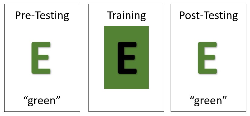
Paired (Repeated) Design
- Key difference: the same people participate in both conditions
## # A tibble: 6 x 2## pre post## <dbl> <dbl>## 1 842. 780.## 2 688. 633.## 3 682. 626.## 4 697. 637.## 5 278. 219.## 6 646. 588.The data are paired
Each row contains the same thing (here, reaction time)
Each row contains data from the same person
Example Output
## ## Paired t-test## ## data: syn_train$pre and syn_train$post## t = 90.76, df = 13, p-value < 0.00000000000000022## alternative hypothesis: true difference in means is not equal to 0## 95 percent confidence interval:## 57.03779 59.81936## sample estimates:## mean of the differences ## 58.42857"There was a significant difference in mean colour naming times between pre- and post-training (t(13) = 90.76, p < .001, Mdiff = 58.43, 95% CI [57.04, 59.82])."
Causality
In our first example, could we conclude that having synaesthesia causes you to pay more attention to language?
In our second example, could we conclude that having training causes you to associate colours with letters?
Causality
In our first example, could we conclude that having synaesthesia causes you to pay more attention to language?
In our second example, could we conclude that having training causes you to associate colours with letters?
Why is this?
That's the t
The t-test quantifies the size of the difference of two means (signal) compared to the error (noise)
Independent samples t-test
Tests means from different entities/participants
Independent or "between-subjects" design
Paired samples t-test
Tests means from the same entities/participants
Repeated or "within-subjects" design
Establishing causality is a function of study design not statistics!
Lab Reports
You can choose either the red or green study to write your report on
- See Lab Report Information on Canvas for more
If you choose the red study (Elliot et al., 2010), you must use and report the results of an independent samples t-test
Lab Reports
You can choose either the red or green study to write your report on
- See Lab Report Information on Canvas for more
If you choose the red study (Elliot et al., 2010), you must use and report the results of an independent samples t-test
Create a composite score out of the three rating scales
Report means, SDs, and t-test result
Include a figure of the results
Will be covered in depth in the next tutorial and practical!